Pre-Integrated Skin Shading

Introduction
Recently, I was implementing skin shading in my engine. The pre-integrated skin shading technique is chosen because it has a low performance cost and does not require another extra pass. The idea is to pre-bake the scattering effect over a ring into a texture for different curvature to look up during run-time. More information can be found in the GPU Pro 2, the SIGGRAPH slides, and also in the presentation of the game "The Oder:1886". Here is the result implemented in my engine (all screen shots are rendered with filmic tone mapping):

The head on the left is lit with Oren-Nayar shading
The head on the right is lit with pre-integrated skin

Curve Approximation for Direct Lighting
In my engine, iOS is one of my target platform, which only have 8 texture unit to use for the OpenGL ES 2.0 API. This is not enough for the pre-integrated skin look up texture because my engine have already used some slots for light map, shadow map, IBL... So I need to find an approximation to the look up texture.

Unfortunately I don't have a Mathematica license at home. So I think may be I can fit the curve manually by inspecting the shape of the curve. So, I started by plotting the graph of the equation:

Here is the shape of the red channel diffusion curve, plotting with N.L(normalized to [0, 1])and r (from 2 to 16):

My idea for approximating the curve is by finding some simple curves first and then interpolate between them like this:

For the light blue line in the above figure, a single straight line can get a close enough approximation:

curve1= saturate(1.95 * NdotL -0.96)

To approximate the dark blue line, I divide it into 2 parts: linear part and quadratic part:

curve0_linear= saturate(1.75* NdotL -0.76)

curve0_quadratic= 0.65*(NdotL^ 2)  + 0.045

blending both linear and quadratic curve will get a curve that is similar to the original function:

curve0= lerp(curve0_quadratic, curve0_linear, NdotL^2)

Now we have 2 curves that is similar to our original function at both end. By mixing them together, we can get something similar to the original function like this:

curve= lerp(curve0, curve1, 1 - (1 - curvature)^4)

By repeating the above steps for the blue and green channels, we can shade the pre-integrated skin without the look up texture. Here is the result:

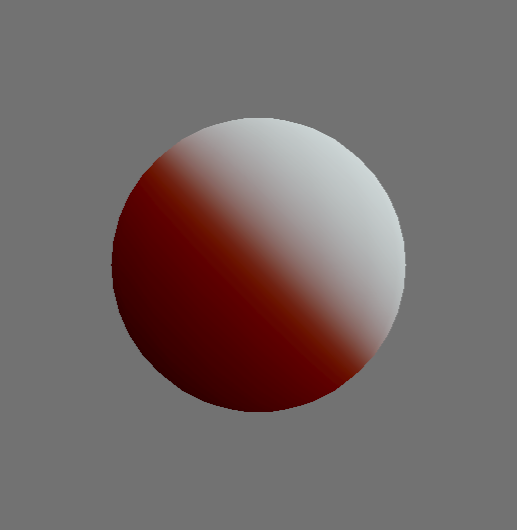
Lit with a single directional light From left to right: r = 2, 4, 8, 16 Upper row: shaded with look up texture Lower row: shaded with approximated function

This is how it looks like when applying to a human head model:

From left to right: shaded with look up texture, approximated function, lambert shader Upper row: shaded with albedo texture applied Lower row: showing only lighting result

For your reference, here is the approximated function I used for the RGB channels:

NdotL = mad(NdotL, 0.5, 0.5); // map to 0 to 1 range
float curva = (1.0/mad(curvature, 0.5 - 0.0625, 0.0625) - 2.0) / (16.0 - 2.0); // curvature is within [0, 1] remap to normalized r from 2 to 16
float oneMinusCurva = 1.0 - curva;
float3 curve0;
{
    float3 rangeMin = float3(0.0, 0.3, 0.3);
    float3 rangeMax = float3(1.0, 0.7, 0.7);
    float3 offset = float3(0.0, 0.06, 0.06);
    float3 t = saturate( mad(NdotL, 1.0 / (rangeMax - rangeMin), (offset + rangeMin) / (rangeMin - rangeMax)  ) );
    float3 lowerLine = (t * t) * float3(0.65, 0.5, 0.9);
    lowerLine.r += 0.045;
    lowerLine.b *= t.b;
    float3 m = float3(1.75, 2.0, 1.97);
    float3 upperLine = mad(NdotL, m, float3(0.99, 0.99, 0.99) -m );
    upperLine = saturate(upperLine);
    float3 lerpMin = float3(0.0, 0.35, 0.35);
    float3 lerpMax = float3(1.0, 0.7 , 0.6 );
    float3 lerpT = saturate( mad(NdotL, 1.0/(lerpMax-lerpMin), lerpMin/ (lerpMin - lerpMax) ));
    curve0 = lerp(lowerLine, upperLine, lerpT * lerpT);
}
float3 curve1;
{
    float3 m = float3(1.95, 2.0, 2.0);
    float3 upperLine = mad( NdotL, m, float3(0.99, 0.99, 1.0) - m);
    curve1 = saturate(upperLine);
}
float oneMinusCurva2 = oneMinusCurva * oneMinusCurva;
float3 brdf = lerp(curve0, curve1, mad(oneMinusCurva2, -1.0 * oneMinusCurva2, 1.0) );

Curve Approximation for Indirect Lighting
In my engine, the indirect lighting is stored in spherical harmonics up to order 2. So the pre-integrated skin BRDF need to be projected into spherical harmonics coefficients and can be store in look up texture just like the presentation of "The Oder:1886" described. One thing to note about the integral range in equation (19) from the paper should be up to π instead of π/2 because to project the coefficients, we need to integrate over the whole sphere domain and the value of D(θ, r) in the lower hemi-sphere may be non zero for small r due to sub-surface scattering, which does not like the clamped cos(θ). So I compute the spherical harmonics coefficient using this:

To make the indirect lighting work on my target platform, an approximate function to this indirect lighting look up texture also need to be found. By using similar methods described above and with some trail and error. Here is my result:

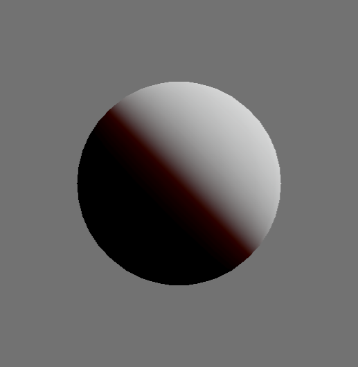
Lit with both directional light and BRDF projected into SH From left to right: r = 2, 4, 8, 16 Upper row: shaded with look up texture Lower row: shaded with approximated function

And applying it to the human head model, but this time the approximation is not close enough and lose a bit of red color:

From left to right: shaded with look up texture, approximated function, lambert shader Upper row: shaded with albedo texture applied Lower row: showing only lighting result

And some code for your reference, where the ZH is the zonal harmonics coefficient:

float curva = (1.0/mad(curvature, 0.5 - 0.0625, 0.0625) - 2.0) / (16.0 - 2.0); // curvature is within [0, 1] remap to r distance 2 to 16
float oneMinusCurva = 1.0 - curva;
// ZH0
{
    float2 remappedCurva = 1.0 - saturate(curva * float2(3.0, 2.7) );
    remappedCurva *= remappedCurva;
    remappedCurva *= remappedCurva;
    float3 multiplier = float3(1.0/mad(curva, 3.2, 0.4), remappedCurva.x, remappedCurva.y);
    zh0 = mad(multiplier, float3( 0.061659, 0.00991683, 0.003783), float3(0.868938, 0.885506, 0.885400));
}
// ZH1
{
    float remappedCurva = 1.0 - saturate(curva * 2.7);    
 float3 lowerLine = mad(float3(0.197573092, 0.0117447875, 0.0040980375), (1.0f - remappedCurva * remappedCurva * remappedCurva), float3(0.7672169, 1.009236, 1.017741));
    float3 upperLine = float3(1.018366, 1.022107, 1.022232);
    zh1 = lerp(upperLine, lowerLine, oneMinusCurva * oneMinusCurva);
}

Result
Putting both the direct and indirect lighting calculation together, with a simple GGX specular, lit by 1 directional light, SH projected indirect light and pre-filtered IBL.

Heads from left to right: shaded with lambert shader, approximated function, look up texture Images from left to right: full shading, direct lighting only, indirect lighting only Upper row: shaded with albedo texture applied Lower row: showing only lighting result

With another lighting environment:

Heads from left to right: shaded with look up texture, approximated function, lambert shader Images from left to right: full shading, direct lighting only, indirect lighting only Upper row: shaded with albedo texture applied Lower row: showing only lighting result

I have uploaded the curvature map for the human head here, look up texture for the direct lighting here and indirect lighting look up texture here. The textures need to be loaded without sRGB conversion. For the indirect lighting texture, I have scale the value so that it fits into an 8-bit texture within 0 to 1 range. So a sample use of the look up textures looks like:

float3 brdf= directBRDF.Sample(samplerLinearClamp, float2(mad(NdotL, 0.5, 0.5), oneOverR)).rgb;
float3 zh0= indirectBRDF_ZH.Sample(samplerLinearClamp, float2(oneOverR, 0.25)).rgb;
float3 zh1= indirectBRDF_ZH.Sample(samplerLinearClamp, float2(oneOverR, 0.75)).rgb;
float remapMin= 0.75;
float remapMax= 1.05;
zh0= zh0 * (remapMax - remapMin) + remapMin;
zh1= zh1 * (remapMax - remapMin) + remapMin;

Conclusion
In this post, I describe a way to find an approximated function for the pre-integrated skin diffusion profile, which gives a similar result for the direct lighting function while losing a bit of red color for the indirect lighting. The down side of fitting the curve manually is when the function is changed a bit, say changing the function input from radial distance to curvature(i.e. from r to 1/r), all the approximate functions need be re-do again (or the conversion need to be done during run-time just like my code snippet above...). Also the shadow scattering described in the original paper is not implemented, so some artifact may be seen at the direct shadow boundary. Overall, the skin shading result is improved compare to shade with Lambert or Oren-Nayar under environment with a strong directional light source.

Reference
[1] SIGGRAPH 2011- Pre-Integrated Skin Shading
http://advances.realtimerendering.com/s2011/Penner%20-%20Pre-Integrated%20Skin%20Rendering%20(Siggraph%202011%20Advances%20in%20Real-Time%20Rendering%20Course).pptx
[2] GPU Pro 2- Pre-Integrated Skin Shading http://www.amazon.com/GPU-Pro-2-Wolfgang-Engel/dp/1568817185
[3]  Crafting a Next-Gen Material Pipeline for The Order: 1886 http://blog.selfshadow.com/publications/s2013-shading-course/rad/s2013_pbs_rad_notes.pdf
[4] GPU Gem 3- Advanced Techniques for Realistic Real-Time Skin Rendering http://http.developer.nvidia.com/GPUGems3/gpugems3_ch14.html
[5] Mathematica and Skin Rendering http://c0de517e.blogspot.jp/2011/09/mathematica-and-skin-rendering.html
[6] Addendum to Mathematica and Skin Rendering http://c0de517e.blogspot.jp/2011/09/mathematica-and-skin-rendering.html
[7] 3D head model by Infinite-Realities http://graphics.cs.williams.edu/data/meshes/head.zip

Recent Update 2014

Overview
It has been a long time since my last post. Life was not that good here in Hong Kong, but I was still working on my engine in spare time. This post will show some of the stuff I have been working on in the past few months.

Shading
On graphics side, the engine is now switched to use physically based shaders with GGX model for specular and Oren-Nayar model for diffuse shading. The GGX model is implemented according to this paper from Unreal Engine 4[1]. While the Oren-Nayar model is implemented according to this paper from tri-Ace[2].

Meshes shaded with physically based shaders with different roughness

Oren-Nayar model is chosen over Lambert model because it takes roughness into account. During shading, for those mesh with roughness map but without normal map, using Oren-Nayar model will show a bit more details.

A mesh shaded without normal map under indirect lighting: From left to right: final result, lighting only, normal, roughness, albedo

Also, a radiosity[3] baking tool was written to calculate the indirect diffuse lighting for static mesh by rendering cube-maps at every light map texel position. The cube maps are then projected into Spherical Harmonics(SH) during the radiosity iteration. And the results are stored in SH luma + average chroma along the vertex normal hemi-sphere (but the chroma format doesn't play well with the texture compression, so may need to find another storage representation in the future...).

Direct + Indirect lighting

Direct lighting only

Lighting only

The indirect specular lighting is baked by capturing reflection probe and pre-filtered with GGX model according to the Unreal Engine 4 paper[1]. Currently only the closest reflection probe is used without parallax correction.

Reflection probes placed within the scene

Shading with pre-filtered cube-map

The indirect diffuse lighting for dynamic mesh is baked into the Irradiance Volumes[4], storing in SH coefficients. The SH coefficients are modified according to roughness described in the tri-Ace paper[2] (This is also done for the SH luma store in the light map for static mesh).

Irradiance Volume samples

Dragon shaded with Irradiance Volume

Shadow
The shadow system is updated to use with a mix of baked and real-time shadow. The light map baker described above calculate a shadow term for the main directional light at each light map texel and stored using signed distance field representation[5][6] (Also, an additional binary shadow term is calculated for each Irradiance Volume sample position for dynamic objects).

Real-time shadow only

baked shadow only

Baked + real-time shadow

For the dynamic soft shadow, Exponential Shadow Map(ESM)[7] is used. But the contact shadow looks too soft, so the shadow term calculated by ESM is raised to the power 4 (i.e. s'= s^4, where s is the shadow attenuation result from ESM) to make it darker.

Potential Visibility Set
A potential visibility set (PVS) baker is written to calculate which meshes are visible to the visibility cells for culling the scene during runtime. A brute force approach is used for baking by taking some sample positions on a given mesh (e.g. vertex position + light map texel position) and then rendering the scene to check whether the visibility cells are visible.

Render without PVS culling	Render with PVS culling	Final rendered result
Another view for the same camera render without PVS culling	Another view for the same camera render with PVS culling	Visibility Cells are placed within the scene for possible camera location

Particles
A basic particle system is implemented which can receive static lighting and receive static shadow. The particle are shaded on CPU using the Irradiance Volumes described above and can be calculated either per vertex, per particle or per emitter.

Particles with lighting and shadow enabled

Self-shadow disabled

The particles can also receive self shadow using the Fourier Opacity Mapping[8]. An opacity map is computed on CPU side for the main directional light which assume each particle is of sphere shape. Then a shadow term can be computed for shading.

Cross platform support
The engine runtime supports 3 different platforms: Windows, Mac, iOS(Editors are Windows only). On Windows, the engine mainly runs with D3D11. An extra OpenGL wrapper was written for Windows to ease the porting to iOS and Mac because it is easier to debug OpenGL with tools like Nsight.

The engine runs on Windows, Mac, iOS platforms

To write cross platform shaders, shaders are written in my own shading language which is similar to HLSL. Those shaders are then parsed by a shader parser generated by Flex and Bison[9] to obtain a syntax tree to output the actual HLSL and GLSL source code.

Final words
Hope you enjoy the above screen shots and wish I can find some time to describe them in details in future posts.

There are some other tasks implemented in the past few months,
such as various editors, audio coding as well as asset hot-reload

Reference
[1] Real Shading in Unreal Engine 4 http://blog.selfshadow.com/publications/s2013-shading-course/karis/s2013_pbs_epic_notes_v2.pdf
[2] Beyond a Simple Physically Based Blinn-Phong Model in Real-time http://research.tri-ace.com/Data/s2012_beyond_CourseNotes.pdf
[3] Radiosity http://en.wikipedia.org/wiki/Radiosity_(computer_graphics)
[4] Irradiance Volumes for Games http://developer.amd.com/wordpress/media/2012/10/Tatarchuk_Irradiance_Volumes.pdf
[5] Improved Alpha-Tested Magnification for Vector Textures and Special Effects http://www.valvesoftware.com/publications/2007/SIGGRAPH2007_AlphaTestedMagnification.pdf
[6] Distance Field Shadows http://udn.epicgames.com/Three/DistanceFieldShadows.html
[7] Exponential Shadow Maps http://research.edm.uhasselt.be/tmertens/papers/gi_08_esm.pdf
[8] Fourier Opacity Mapping http://sebastien.hillaire.free.fr/index.php?option=com_content&view=article&id=61&Itemid=72
[9] Flex and Bison http://aquamentus.com/flex_bison.html

Transforming points in unit square with p-norm

Introduction
Continue with previous post talking about some little tricks I used when implementing the animation editor. This time, I will talk about another maths problem when implementing the directional blend node in the animation tree editor. In this node, it blends 5 different animations(i.e. forward, backward, left, right and center) according to the current direction:

blending 5 different animation according to the current direction

And the UI of this node has a square input region like this for artist to preview how those animations are blended together:

So, to compute a blended output, we need to transform the points in the square region to a rhombus, and then we can use barycentric coordinates to determine the blend weight for blending:

Transform the current direction for computing the blend weight

p-norm
After searching google for a while, something called Lp-space has shown up with the following figures which looks similar to what I need:

Showing "unit circle" with different p-norm

All of the above figures are showing a "unit circle" (i.e. the vectors are of unit-length), but measured with different p-norms. The definition of p-norm is:

This equation describe the length of a vector. When p=2, it is the Euclidean norm that we normally use. Our goal is to transform points inside the unit square to the rhombus, in other words, we want the transformed points having the same length as before the transformation but measured with different p-norm, using p=1 after the transformation and p=infinity before transformation. In other words, we have (assume only dealing with the 2D case, and only consider points in the first quadrant):

, where v=(x, y) is the original point and v'=(x', y') is the transformed point.

Mapping the points
As our target is to find a function to transform the points, having only the above equation is not enough as there are infinitely many way to transform the point that satisfy the above equation. So we need another equation to find a unique solution, the idea is to have the transformed point, original point and the origin are lying on the same straight line(i.e. having the same slope), which gives another equation:

By solving the above equations, which gives the transform functions:

Taking into account those points in other quadrant and special case, which gives the final mapping functions:

However, taking the limit p to infinity and compute it with Wolfram Alpha does not gives any useful result... So I just take p=10 (taking a too large value will result in floating point precision problem...). Here is the plot of how the points are transformed/squeezed into the rhombus:

Graph showing how points are transformed from square to rhombus 

Although the function cannot transformed the points into a perfect rhombus, it does not have too much artifact when used for animation blending.

Conclusion
In this post, I have described how to map points inside a unit square to a "rhombus" which used for animation blending. But the problem is not completely solved as I am not taking the limit of p to infinity, and there are some power function in the transformation which is not fast... But this is enough for calculating the blend weight of the animations.

Reference
[1] Lp space: http://en.wikipedia.org/wiki/Lp_space